Receiver operator curve

roc_curve() constructs the full ROC curve and returns a tibble. See roc_auc() for the area under the ROC curve.

Usage

roc_curve(data, ...)

# S3 method for data.frame
roc_curve(
  data,
  truth,
  ...,
  na_rm = TRUE,
  event_level = yardstick_event_level(),
  case_weights = NULL,
  options = list()
)

Arguments

data

A data.frame containing the columns specified by truth and ....

...

A set of unquoted column names or one or more dplyr selector functions to choose which variables contain the class probabilities. If truth is binary, only 1 column should be selected, and it should correspond to the value of event_level. Otherwise, there should be as many columns as factor levels of truth and the ordering of the columns should be the same as the factor levels of truth.

truth

The column identifier for the true class results (that is a factor). This should be an unquoted column name although this argument is passed by expression and supports quasiquotation (you can unquote column names). For _vec() functions, a factor vector.

na_rm

A logical value indicating whether NA values should be stripped before the computation proceeds.

event_level

A single string. Either "first" or "second" to specify which level of truth to consider as the "event". This argument is only applicable when estimator = "binary". The default uses an internal helper that defaults to "first".

case_weights

The optional column identifier for case weights. This should be an unquoted column name that evaluates to a numeric column in data. For _vec() functions, a numeric vector, hardhat::importance_weights(), or hardhat::frequency_weights().

options

[deprecated]

No longer supported as of yardstick 1.0.0. If you pass something here it will be ignored with a warning.

Previously, these were options passed on to pROC::roc(). If you need support for this, use the pROC package directly.

Value

A tibble with class roc_df or roc_grouped_df having columns .threshold, specificity, and sensitivity.

Details

roc_curve() computes the sensitivity at every unique value of the probability column (in addition to infinity and minus infinity).

There is a ggplot2::autoplot() method for quickly visualizing the curve. This works for binary and multiclass output, and also works with grouped data (i.e. from resamples). See the examples.

Multiclass

If a multiclass truth column is provided, a one-vs-all approach will be taken to calculate multiple curves, one per level. In this case, there will be an additional column, .level, identifying the "one" column in the one-vs-all calculation.

Relevant Level

There is no common convention on which factor level should automatically be considered the "event" or "positive" result when computing binary classification metrics. In yardstick, the default is to use the first level. To alter this, change the argument event_level to "second" to consider the last level of the factor the level of interest. For multiclass extensions involving one-vs-all comparisons (such as macro averaging), this option is ignored and the "one" level is always the relevant result.

See also

Compute the area under the ROC curve with roc_auc().

Other curve metrics: gain_curve(), lift_curve(), pr_curve()

Author

Max Kuhn

Examples

# ---------------------------------------------------------------------------
# Two class example

# `truth` is a 2 level factor. The first level is `"Class1"`, which is the
# "event of interest" by default in yardstick. See the Relevant Level
# section above.
data(two_class_example)

# Binary metrics using class probabilities take a factor `truth` column,
# and a single class probability column containing the probabilities of
# the event of interest. Here, since `"Class1"` is the first level of
# `"truth"`, it is the event of interest and we pass in probabilities for it.
roc_curve(two_class_example, truth, Class1)
#> # A tibble: 502 × 3
#>    .threshold specificity sensitivity
#>         <dbl>       <dbl>       <dbl>
#>  1 -Inf           0                 1
#>  2    1.79e-7     0                 1
#>  3    4.50e-6     0.00413           1
#>  4    5.81e-6     0.00826           1
#>  5    5.92e-6     0.0124            1
#>  6    1.22e-5     0.0165            1
#>  7    1.40e-5     0.0207            1
#>  8    1.43e-5     0.0248            1
#>  9    2.38e-5     0.0289            1
#> 10    3.30e-5     0.0331            1
#> # ℹ 492 more rows

# ---------------------------------------------------------------------------
# `autoplot()`

# Visualize the curve using ggplot2 manually
library(ggplot2)
library(dplyr)
roc_curve(two_class_example, truth, Class1) %>%
  ggplot(aes(x = 1 - specificity, y = sensitivity)) +
  geom_path() +
  geom_abline(lty = 3) +
  coord_equal() +
  theme_bw()


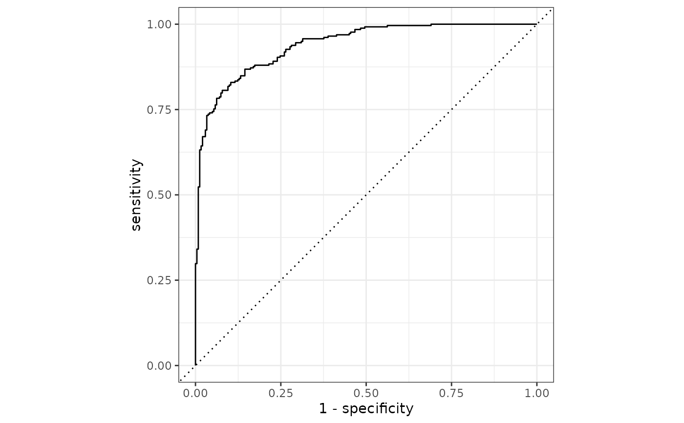# Or use autoplot
autoplot(roc_curve(two_class_example, truth, Class1))


if (FALSE) {

# Multiclass one-vs-all approach
# One curve per level
hpc_cv %>%
  filter(Resample == "Fold01") %>%
  roc_curve(obs, VF:L) %>%
  autoplot()

# Same as above, but will all of the resamples
hpc_cv %>%
  group_by(Resample) %>%
  roc_curve(obs, VF:L) %>%
  autoplot()
}